Machine learning to segment neutron images

Machine learning to segment neutron images

Anders Kaestner, Beamline scientist - Neutron Imaging

Laboratory for Neutron Scattering and Imaging
Paul Scherrer Institut

Lecture outline

In this lecture about machine learning to segment neutron images we will cover the following topics

1. Introduction
2. Limited data problem
3. Unsupervised segmentation
4. Supervised segmentation
5. Final problem: Segmenting root networks using convolutional NNs
6. Future Machine learning challenges in NI

Getting started

If you want to run the notebook on your own computer, you'll need to perform the following step:

• You will need to install Anaconda
• Clone the lecture repository (in the location you'd like to have it)

  git clone https://github.com/ImagingLectures/MLSegmentation4NI.git
  

• Enter the folder 'MLSegmentation'
• Create an environment for the notebook

  conda env create -f environment. yml -n MLSeg4NI
  

• Enter the environment

  conda env activate MLSeg4NI
  

• Start jupyter and open the notebook lecture/ML4NeutronImageSegmentation.ipynb

• Use the notebook

• Leave the environment

  conda env deactivate
  

Importing needed modules

This lecture needs some modules to run. We import all of them here.

import matplotlib.pyplot as plt
import seaborn           as sn
import numpy             as np
import pandas            as pd
import skimage.filters   as flt
import skimage.io        as io
import matplotlib        as mpl

from sklearn.cluster     import KMeans
from sklearn.neighbors   import KNeighborsClassifier
from sklearn.metrics     import confusion_matrix
from sklearn.datasets    import make_blobs

from matplotlib.colors   import ListedColormap
from matplotlib.patches  import Ellipse
from lecturesupport      import plotsupport as ps

import scipy.stats       as stats
import astropy.io.fits   as fits

import keras.metrics     as metrics
import keras.losses      as loss
import keras.optimizers  as opt
from keras.models        import Model
from keras.layers        import Input, Conv2D, MaxPooling2D, UpSampling2D, concatenate

%matplotlib inline


from IPython.display import set_matplotlib_formats
set_matplotlib_formats('svg', 'png')
#plt.style.use('seaborn')
mpl.rcParams['figure.dpi'] = 300

Using TensorFlow backend.

import importlib
importlib.reload(ps);

Introduction

In this introduction part we give a starting point for the lecture. With topics like.

• Introduction to neutron imaging

  • Some words about the method
  • Contrasts

• Introduction to segmentation

  • What is segmentation
  • Noise and SNR

• Problematic segmentation tasks

  • Intro
  • Segmentation problems in neutron imaging

From these topics we will go into looking at how different machine learning techniques can be used to segment images. An in particular images obtained in neutron imaging experiments

What is an image?

In this lecture we are going to analyze the contents of images, but first lets define what an image is.

A very abstract definition:

• A pairing between spatial information (position)
• and some other kind of information (value).

In most cases this is a two- or three-dimensional position (x,y,z coordinates) and a numeric value (intensity)

In reality it can be many things like a picture, a radiograph, a matrix presentation of a raster scan and so on. In the case of volume images we are talking about volume representations like a tomography or time series like movies.

```{figure} figures/imagesampling.pdf

scale: 75%

The real world is sampled into discrete images with limited extent. ```

Science and Imaging

Images are great for qualitative analyses since our brains can quickly interpret them without large programming investements.

This is also the reason why image processing can be very frustrating. Seeing a feature in the image may be obvious to the human eye, but it can be very hard to write an algorithm that makes the same conclusion. In particular, when you are using traditional image processing techniques. This is an classic area for machine learning, these methods are designed and trained to recognize patterns and features in the images. Still, they can only perform well on the type of data they are trained with.

Proper processing and quantitative analysis is however much more difficult with images.

• If you measure a temperature, quantitative analysis is easy, $T=50K$.
• If you measure an image it is much more difficult and much more prone to mistakes,
  • subtle setup variations may break you analysis process,
  • and confusing analyses due to unclear problem definition

Furthermore in image processing there is a plethora of tools available

• Thousands of algorithms available
• Thousands of tools
• Many images require multi-step processing
• Experimenting is time-consuming

Some word about neutron imaging

Neutron imaging is a method based on transmission of the neutron radiation through a sample, i.e. the fundamental information is a radiograph. In this sense it is very much similar to the more known x-ray imaging. The basic outline in the figure below show the components source, collimator, sample, and detector. The neutron beam is slightly divergent, but it can mostly be approximated by a parallel beam.

```{figure} figures/collimator.pdf

scale: 75%

Schematic transmission imaging setup. ```

The intensity in a radiographic image proportional to the amount of radiation that remains after it was transmitted through the sample.

The transmitted radiation is described by Beer-Lambert's law which in its basic form looks like

$$I=I_0\cdot{}e^{-\int_L \mu{}(x) dx}$$

```{figure} figures/AttenuationLaw.pdf

scale: 30%

Transmission plot through a sample. ```

Where $\mu(x)$ is the attenuation coefficient of the sample at position x. This equation is a simplification as no source has a uniform spectrum and the attenuation coefficient depends on the radiation energy. We will touch the energy dispersive property in one of the segmentation examples later.

Single radiographs are relatively rare. In most experiments the radiographs are part of a time series aquisition or projections for the 3D tomography reconstuction. In this lecture we are not going very much into the details about the imaging method as such. This is a topic for other schools that are offered.

Image types obtained with neutron imaging

Fundamental information	Additional dimensions	Derived information
2D Radiography	Time series	q-values
3D Tomography	Spectra	strain
		Crystal orientation

Neutron imaging contrast

The integral of Beer-Lambert's law turns into a sum for simple material compositions like in the sample in the figure below

```{figure} figures/porous_media_sand.pdf

scale: 50%

The transmission through a sample can be divied into contributions for each material.

The amount of radiation passing through the sample depends on the attenuation coefficients which are material and radiation specific. The periodic systems below illustrate how diffent elements attenuate for neutrons and X-rays

```{figure} figures/Periodic_table_neutron.pdf
---
scale: 75%
---
Attenuation coefficients for thermal neutrons.

```{figure} figures/Periodic_table_Xray.pdf

scale: 75%

Attenuation coefficients for X-rays. ```

---

Transmission through sample	X-ray attenuation	Neutron attenuation

Measurements are rarely perfect

There is no perfect measurement. This is also true for neutron imaging. The ideal image is the sample is distorted for many reasons. The figure below shows how an image of a sample can look after passing though the acquisition system. These quailty degradations will have an impact on the analysis of the image data. In some cases, it is possible to correct for some of these artifacts using classing image processing techniques. There are however also cases that require extra effort to correct the artifacts.

```{figure} figures/imperfect_imaging_system.pdf

scale: 75%

Schematic showing the error contributions in an imperfect imaging system. ```

Factors affecting the image quality

The list below provides some factors that affect the quality of the acquired images. Most of them can be handled by changing the imaging configuration in some sense. It can however be that the sample or process observed put limitiations on how much the acquisition can be tuned to obtain the perfect image.

• Resolution (Imaging system transfer functions)
• Noise
• Contrast
• Inhomogeneous contrast
• Artifacts

Resolution

The resolution is primarily determined optical transfer function of the imaging system. The actual resolution is given by the extents of the sample and how much the detector needs to capture in one image. This gives the field of view and given the number pixels in the used detector it is possible to calculate the pixel size. The pixel size limits the size of the smallest feature in the image that can be detected. The scintillator, which is used to convert neutrons into visible light, is chosen to

1. match the sampling rate given by the pixel size.
2. provide sufficient neutron capture to obtain sufficient light output for a given exposure time.

Noise

An imaging system has many noise sources, each with its own distribution e.g.

1. Neutron statistics - how many neutrons are collected in a pixel. This noise is Poisson distributed.
2. Photon statistics - how many photons are produced by each neutron. This noise is also Poisson distributed.
3. Thermal noise from the electronics which has a Gaussian distribution.
4. Digitation noise from converting the charges collected for the photons into digital numbers that can be transfered and stored by a computer, this noise has a binominal distribution.

The neutron statistics are mostly dominant in neutron imaging but in some cases it could also be that the photon statistics play a role.

Contrast

The contrast in the sample is a consequence of

1. how well the sample transmits the chosen radiation type. For neutrons you obtain good contrast from materials containing hydrogen or lithium while many metals are more transparent.
2. the amount of a specific element or material represented in a unit cell, e.g. a pixel (radiograph) or a voxel (tomography).

The objective of many experiments is to quantify the amount of a specific material. This could for example be the amount of water in a porous medium.

Good contrast between different image features is important if you want to segment them to make conclusions about the image content. Therefore, the radiation type should be chosen to provide the best contrast between the features.

Inhomogeneous contrast

The contrast in the raw radiograph depends much on the beam profile. These variations are easily corrected by normalizing the images by an open beam or flat field image.

• Biases introduced by scattering Scattering is the dominant interaction for many materials use in neutron imaging. This means that neutrons that are not passing straight though the sample are scattered and contribute to a background cloud of neutrons that build up a bias of neutron that are also detected and contribute to the

• Biases from beam hardening is a problem that is more present in x-ray imaging and is caused by that fact that the attenuation coefficient depends on the energy of the radiation. Higher energies have lower attenuation coefficient, thus will high energies penetrate the thicker samples than lower energies. This can be seen when a polychromatic beam is used.

Artifacts

Many images suffer from outliers caused by stray rays hitting the detector. Typical artefacts in tomography data are

• Lines, which are caused by outlier spots that only appear in single projections. These spot appear as lines in the reconstructed images.
• Rings are caused by stuck pixels which have the same value in a projections.

Introduction to segmentation

The basic task of segmentation is to identify regions of pixels with similar properties. This can be on different levels of abstraction. The lowest level is to create segments of pixels based on their pixel values like in the LANDSAT image below.

```{figure} figures/landsat_example.pdf

scale: 50%

Segmentation of a satelite image to identify different land types. ```

This type of segmentation sometimes be done with the help of a histogram that shows the distribution of values in the image.

Different types of segmentation

When we talk about image segmentation there are different meanings to the word. In general, segmenation is an operation that marks up the image based on pixels or pixel regions. This is a task that has been performed since beginning of image processing as it is a natural step in the workflow to analyze images - we must know which regions we want to analyze and this is a tedious and error prone task to perform manually. Looking at the figure below we two type of segmentation.

• Object detection - identifies regions containing an object. The exact boundary does not matter so much here. We are only interested in a bounding box.

• Semantic segmentation - classifies all the pixels of an image into meaningful classes of objects. These classes are “semantically interpretable” and correspond to real-world categories. For instance, you could isolate all the pixels associated with a cat and color them green. This is also known as dense prediction because it predicts the meaning of each pixel.

• Instance segmentation - Identifies each instance of each object in an image. It differs from semantic segmentation in that it doesn’t categorize every pixel. If there are three cars in an image, semantic segmentation classifies all the cars as one instance, while instance segmentation identifies each individual car.

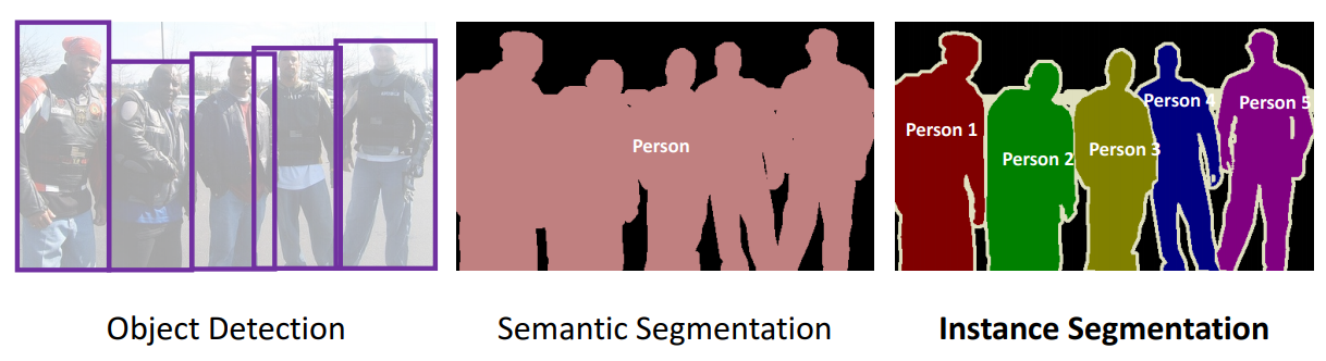
Basic segmentation: Applying a threshold to an image

Start out with a simple image of a cross with added noise

$$ I(x,y) = f(x,y) $$

Here, we create a test image with two features embedded in uniform noise; a cross with values in the order of '1' and background with values in the order '0'. The figure below shows the image and its histogram. The histogram helps us to see how the graylevels are distributed which guides the decision where to put a threshold that segments the cross from the background.

fig,ax = plt.subplots(1,2,figsize=(12,6))
nx = 5; ny = 5;
# Create the test image
xx, yy   = np.meshgrid(np.arange(-nx, nx+1)/nx*2*np.pi, np.arange(-ny, ny+1)/ny*2*np.pi)
cross_im = 1.5*np.abs(np.cos(xx*yy))/(np.abs(xx*yy)+(3*np.pi/nx)) + np.random.uniform(-0.25, 0.25, size = xx.shape)       

# Show it
im=ax[0].imshow(cross_im, cmap = 'hot'); ax[0].set_title("Image")
ax[1].hist(cross_im.ravel(),bins=10); ax[1].set_xlabel('Gray value'); ax[1].set_ylabel('Counts'); ax[1].set_title("Histogram");

Applying a threshold to an image

By examining the image and probability distribution function, we can deduce that the underyling model is a whitish phase that makes up the cross and the darkish background

Applying the threshold is a deceptively simple operation

$$ I(x,y) = \begin{cases} 1, & f(x,y)\geq0.40 \\ 0, & f(x,y)<0.40 \end{cases}$$

threshold = 0.4; thresh_img = cross_im > threshold
fig,ax = plt.subplots(1,2,figsize=(12,6))
ax[0].imshow(cross_im, cmap = 'hot', extent = [xx.min(), xx.max(), yy.min(), yy.max()]); ax[0].set_title("Image")
ax[0].plot(xx[np.where(thresh_img)]*0.9, yy[np.where(thresh_img)]*0.9,
           'ks', markerfacecolor = 'green', alpha = 0.5,label = 'Threshold', markersize = 22); ax[0].legend(fontsize=12);
ax[1].hist(cross_im.ravel(),bins=10); ax[1].axvline(x=threshold,color='r',label='Threshold'); ax[1].legend(fontsize=12); 
ax[1].set_xlabel('Gray value'); ax[1].set_ylabel('Counts'); ax[1].set_title("Histogram");

In this fabricated example we saw that thresholding can be a very simple and quick solution to the segmentation problem. Unfortunately, real data is often less obvious. The features we want to identify for our qantitative analysis are often obscured be different other features in the image. They may be part of the setup of caused by the acquisition conditions.

Noise and SNR

Any measurement has a noise component and this noise has to be dealt with in some way when the image is to be segmented. When the noise is not handled correctly it will cause many misclassified pixels. The noise strength of measured using the signal to noise ratio SNR. It is defined as the ratio between signal average and signal standard deviation.

The noise in neutron imaging mainly originates from the amount of captured neutrons.

This noise is Poisson distributed and the signal to noise ratio is

$$SNR=\frac{E[x]}{s[x]}\sim\frac{N}{\sqrt{N}}=\sqrt{N}$$

where N is the number of captured neutrons. The figure below shows two neutron images acquired at 0.1s and 10s respectively. The plot shows the signal to noise ratio obtained for different exposure times.

```{figure} figures/snrhanoi.pdf

scale: 75%

Signal to noise ratio for radiographies acqired with different exposure times. ``` The signal to noise ratio can be improved by increasing the number of neutrons per pixel. This can be achived through increasing

• Neutron flux - this is usually relatively hard as the neutron sources operate with the parameters it is designed for. There is a posibilty by changing the neutron aperture, but has an impact of the beam quality.
• Exposure time - the exposure time can be increased but in the end there is a limitation on how much this can be used. Beam time is limited which means the experiment must be finished in a given time. There is also an upper limit on the exposure time defined by the observed sample or process when it changes over time. Too long exposure times will result in motion artefacts.
• Pixel size - increasing the pixel size means that neutrons are collected over a greater area and thus more neutrons are captured during the exposure. The limit on how much you can increase the pixel size is defined by the smallest features you want to detect.
• Detector material and thickness - the number of captured neutrons depends on the scintillator material and how thick it is. The thickness does however have an impact on the resolution. Therefore scintillator thickness and pixel size often increase in parallel as there is no point in oversampling a smooth signal to much.

In the end, there are many parameters that combined results in the SNR you obtain. These parameters are tuned to match the experiment conditions. Filtering techniques can help to increase the SNR still it is too low for your quantitative analysis.

Problematic segmentation tasks

Segmentation is rarely an obvious task. What you want to find is often obscured by other image features and unwanted artefacts from the experiment technique. If you take a glance at the painting by Bev Doolittle, you quickly spot the red fox in the middle. Looking a little closer at the painting, you'll recognize two indians on their spotted ponies. This example illustrates the problems you will encounter when you start to work with image segmentation.

```{figure} figures/doolittle_woodlandencounter.png

scale: 75%

Cases making the segmentation task harder than just applying a single thresshold. ```

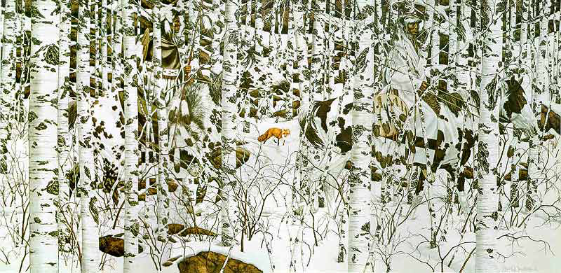
Woodland Encounter Bev Doolittle

Typical image features that makes life harder

The basic segmentation shown in the example above can only be used under good conditions when the classes are well separated. Images from many experiments are unfortunately not well-behaved in many cases. The figure below shows four different cases when an advanced technique is needed to segment the image. Neutron images often show a combination of all cases.

```{figure} figures/trickycases.pdf

scale: 75%

Cases making the segmentation task harder than just applying a single thresshold. ```

The impact on the segmentation performance of all these cases can be reduced by proper experiment planning. Still, sometimes these improvements are not fully implemented in the experiment to be able to fulfill other experiment criteria.

In neutron imaging you see all these image phenomena.

Limited data problem

Machine learning methods require a lot of training data to be able to build good models that are able to detect the features they are intended to.

Different types of limited data:

• Few data points or limited amounts of images

This is very often the case in neutron imaging. The number of images collected during an experiment session is often very low due to the long experiment duration and limited amount of beam time. This makes it hard to develop segmentation and analysis methods for single experiments. The few data points problem can partly be overcome by using data from previous experiment with similar characteristics. The ability to recycle data depends on what you want to detect in the images.

• Unbalanced data

Unbalanced data means that the ratio between the data points with features you want detect and the total number data points is several orders of magnitude. E.g roots in a volume like the example we will look at later in this lecture. There is even a risk that the distribution of the wanted features is overlapped by the dominating background distribution.

```{figure} figures/classunbalance.pdf

scale: 100%

Two cases of unblanaced data; (a) the classes are well separated and the feature class is clearly visible in the tail distribution of the background and (b) the feature class is embeded in the background making it hard to detect. ```

Case (a) can most likely be segmented using one of the many histogram based thresholding methods proposed in literature. Case (b) is much harder to segment as the target features have similar gray levels as the background. This case requires additional information to make segmentation posible.

• Little or missing training data

A complete set of training data contains both input data and labelled data. The input data is easy to obtain, it is the images you measured during your experiment. The labelled data is harder to get as it is a kind of chicken and egg problem. In particular, if your experiment data is limited. In that case, you would have to mark-up most of the available data to obtain the labeled data. Which doesn't make sense because

• then you'd already solved the task before even starting to train your segmentation algorithm.
• An algorithm based on learning doesn't improve the results, it only make it easier to handle large amounts of data.

Training data from NI is limited

The introducing words about limited data essentially describes the problems that arise in neutron imaging. There are several reasons for this. Some are:

• Long experiment times
• Few samples
• Some recycling from previous experiments is posible.

The experiment times are usually rather long which results in only few data sets per experiment. In some cases there is the advantage that there are plenty experiments over the years that produced data with similar characteristics. These experiments can be used in a pool of data.

Augmentation to increase training data

Obtaining more experiment data is mostly relatively hard in neutron imaging. The available time is very limited. Still, many supervised analysis methods require large data sets to perform reliably. A method to improve this situation is to use data augmentation. The figure below shows some examples of augmentations of the same image. You can also add noise and modulate the image intensity to increase the variations further.

```{figure} figures/Augmentations.pdf

scale: 100%

A retinal image modified using different augmentation techniques (source: https://drive.grand-challenge.org/DRIVE/) prepared by Gian Guido Parenza. ```

Data augmentation is a method modify your exisiting data to obtain variations of it.

Augmentation will be used to increase the training data in the root segmenation example in the end of this lecture.

Simulation to increase training data

A further way to increase training data is to build a model of the features you want to train on. This approach has the advantage that you know where to look for the features which means the tedious annotation task is reduced to a minimum. The work rather lies in building a relieable model that should reflect the characteristics of features you want to segments. Once a valid model is built, it is easy to generate masses of data under variuos conditions.

• Geometric models
• Template models
• Physical models

Both augmented and simulated data should be combined with real data.

Transfer learning

Many machine learning techniques also have the ability to remember what they learned before. This effect can be used to improve the performance also when little data is available from the current experiment.

Transfer learning is a technique that uses a pre-trained network to

• Speed up training on your current data
• Support in cases of limited data
• Improve network performance

Usually, the input and downsampling part of the network is used from the pre trained network. It can be set as constant or trainable. The upsampling and output will be trained with new data from your current data set. Transfer learning will be covered in the root segmentation example in the end of this lecture.

Unsupervised segmentation

Unsupervised segmentation method tries to make sense of the that without any prior knowledge. They may need an initialization parameter telling how many classes are expected in the data, but beyond that you don't have to provide much more information.

Introducing clustering

With clustering methods you aim to group data points together into a limited number of clusters. Here, we start to look at an example where each data point has two values. The test data is generated using the make_blobs function.

test_pts = pd.DataFrame(make_blobs(n_samples=200, random_state=2018)[
                        0], columns=['x', 'y'])
plt.plot(test_pts.x, test_pts.y, 'r.');

The generated data set has two obvoius clusters, but if look closer it is even possible to identify three clusters. We will now use this data to try the k-means algorithm.

k-means

The k-means algorithm is one of the most used unsupervised clustering method.

It is an iterative method that starts with a label image where each pixel has a random label assignment. Each iteration involves the following steps:

1. Compute current centroids based on the o current labels
2. Compute the value distance for each pixel to the each centroid. Select the class which is closest.
3. Reassign the class value in the label image.
4. Repeat until no pixels are updated.

The distance from pixel i to centroid j is usually computed as $||p_i - c_j||_2$.

```{figure} figures/FuzzyCMeans.pdf

scale: 100%

Flow chart for the k-means clustering iterations. ```

The user only have to provide the number of classes the algorithm shall find.

Note The algorithm will find exactly the number you ask it to, it doesn't care if it makes sense!

Basic clustering example

In this example we will use the blob data we previously generated and to see how k-means behave when we select different numbers of clusters.

N=3
fig, ax = plt.subplots(1,N,figsize=(18,4.5))

for i in range(N) :
    km = KMeans(n_clusters=i+2, random_state=2018); n_grp = km.fit_predict(test_pts)
    ax[i].scatter(test_pts.x, test_pts.y, c=n_grp)
    ax[i].set_title('{0} groups'.format(i+2))

When we select two clusters there is a natural separation between the two clusters we easily spotted by just looking at the data. When the number of clusters is increased to three, we again see a cluster separation that makes sense. Now, when the number of clusters is increased yet another time we see that one of the clusters is split once more. This time it is how ever questionable if the number of clusters makes sense. From this example, we see that it is important to be aware of problems related to over segmentation.

Add spatial information to k-means

It is important to note that k-means by definition is not position sensitive. Clustering is by definition not position sensitive, mainly measures distances between values and distributions. The position can however be included as additional components in the data vectors. You can also add neighborhood information using filtered images as additionals components of the feature vectors.

orig = fits.getdata('../data/spots/mixture12_00001.fits')[::4,::4]
fig,ax = plt.subplots(1,6,figsize=(18,5)); x,y = np.meshgrid(np.linspace(0,1,orig.shape[0]),np.linspace(0,1,orig.shape[1]))
ax[0].imshow(orig, vmin=0, vmax=4000), ax[0].set_title('Original')
ax[1].imshow(x), ax[1].set_title('x-coordinates')
ax[2].imshow(y), ax[2].set_title('y-coordinates')
ax[3].imshow(flt.gaussian(orig, sigma=5)), ax[3].set_title('Weighted neighborhood')
ax[4].imshow(flt.sobel_h(orig),vmin=0, vmax=0.001),ax[4].set_title('Horizontal edges')
ax[5].imshow(flt.sobel_v(orig),vmin=0, vmax=0.001),ax[5].set_title('Vertical edges');

Scaling the values is very important when you use these additional feature vectors. Otherwise, some vectors will dominate others.

When can clustering be used on images?

Clustering and in particular k-means are often used for imaging applications.

• Single images

It does not make much sense to segment single images using k-means. This would result in thresholding similar to the one provided by Otsu's method. If you, however, add spatial information like edges and positions it starts be interesting to use k-means for a single image.

• Bimodal data

In recent years, several neutron imaging instruments have have installed an X-ray source to provide complementary information to the neutron images. This is a great mix of information for k-means based segmenation. Another type of bimodal data is when a grating interferometry setup is used. This setup provides three images revealing different aspects of the samples. Again, here it a great combination as these data are

• Spectrum data

Many materials have a characteristic response the neutron wavelength. This is used in many materials science experiments, in particular experiments performed at pulsed neutron sources. The data from such experiments result in a spectrum response for each pixel. This means each pixel can be a vector of >1000 elements.

Clustering applied to wavelength resolved imaging

The imaging technique

Samples	Spectrum	Wavelength scan

Images courtesy of S. Peetermans

The data

In this example we use a time of flight transmission spectrum from an assembly of six rectangular steel blocks produced by means of additive manufactoring. The typical approach to analyse this kind of information is to select some regions of interest and compute the average spectra from these regions. The average spectra are then analyzed using single Bragg edge fitting methods or Rietveld refinement.

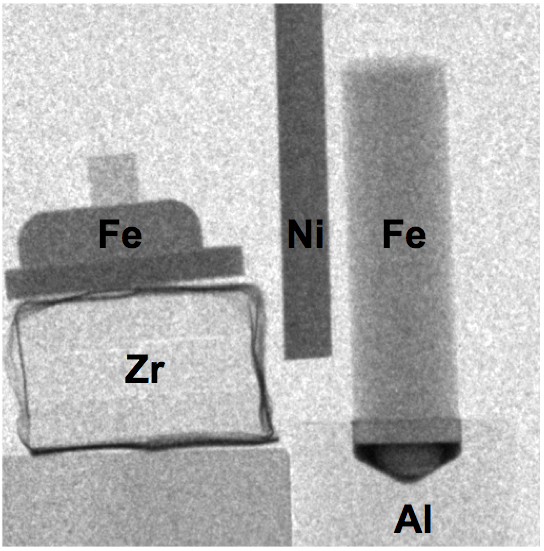
Here, we will explore the posibility to identify regions with similar spectra using k-means clustering. The data is provided on the repository and has the dimensions 128x128x661, where the first to dimensions reflect the image size and the last is th number of time bins of the time of flight spectrum. This is a downsized version of the original data which has 512x512 image frames. Each frame has a relatively low signal to noise ratio, therefore we use the average image wtof to show the image contents.

tof  = np.load('../data/tofdata.npy')
wtof = tof.mean(axis=2)
plt.imshow(wtof,cmap='gray'); 
plt.title('Average intensity all time bins');

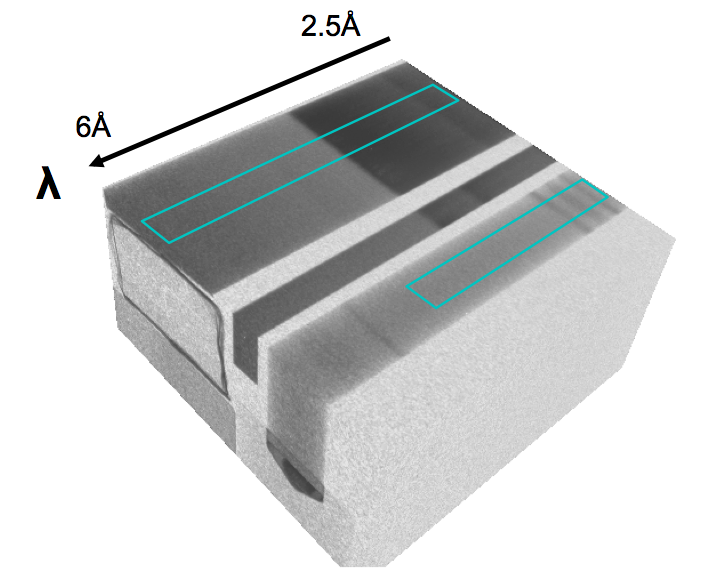
Looking at the spectra

The average image told us that there are six sample regions, some void, and some spacers separating the samples. Now you might think, "easy" just apply some thresholds on the image and you have identified these regions. Now, the pixels in this image are represented by over 600 spectrum samples which reveal a different story. The sample was exposed to a surface treatment and we expect to locate regions within the samples. Given this information it is much harder to identify the regions of interest.

fig, ax= plt.subplots(1,2,figsize=(12,5))
ax[0].imshow(wtof,cmap='gray'); ax[0].set_title('Average intensity all time bins');
ax[0].plot(57,3,'ro'), ax[0].plot(15,30,'bo'), ax[0].plot(79,90,'go'); ax[0].plot(100,120,'co');
ax[1].plot(tof[30,15,:],'b', label='Sample'); ax[1].plot(tof[3,57,:],'r', label='Background'); ax[1].plot(tof[90,79,:],'g', label='Spacer'); ax[1].legend();ax[1].plot(tof[120,100,:],'c', label='Sample 2');

These plots are very noisy and it may even be hard to identify regions with the same spectrum. This is where k-means may come to you help.

Reshaping

The k-means requires vectors for each feature dimension, not images as we have in this data set. Therefore, we need to reshape our data. The reshaping is best done using the numpy array method reshape like this:

tofr=tof.reshape([tof.shape[0]*tof.shape[1],tof.shape[2]])
print("Input ToF dimensions",tof.shape)
print("Reshaped ToF data",tofr.shape)

Input ToF dimensions (128, 128, 661)
Reshaped ToF data (16384, 661)

The reshaped data tofr now has the dimensions 16384x661, i.e. each 128x128 pixel image has been replaced by a vector with the length 16384 elements. The number of time bins still remains the same. The reshapemethod is a cheap operation as it only changes the elements of the dimension vector and doesn't rearrange the data in memory.

Setting up and running k-means

When we set up k-means, we merely have to select the number of clusters. The choice depends on many factors. Particularly in this case with data points containing a large number of values we have a great degree of freedom in what could be considered the correct result. Thus we should ask ourselves what we expect from the clustering.

• We can clearly see that there is void on the sides of the specimens.
• There is also a separating band between the specimens.
• Finally we have to decide how many regions we want to find in the specimens. Let's start with two regions with different characteristics.

km = KMeans(n_clusters=4, random_state=2018)     # Random state is an initialization parameter for the random number generator
c  = km.fit_predict(tofr).reshape(tof.shape[:2]) # Label image
kc = km.cluster_centers_.transpose()             # cluster centroid spectra

Results from the first try

fig,axes = plt.subplots(1,3,figsize=(18,5)); axes=axes.ravel()
axes[0].imshow(wtof,cmap='viridis'); axes[0].set_title('Average image')
p=axes[1].plot(kc);                  axes[1].set_title('Cluster centroid spectra'); axes[1].set_aspect(tof.shape[2], adjustable='box')
cmap=ps.buildCMap(p) # Create a color map with the same colors as the plot

im=axes[2].imshow(c,cmap=cmap); plt.colorbar(im);
axes[2].set_title('Cluster map');
plt.tight_layout()

An advantage of the k-means is that it computes the centroid spectra for you as you go along. This means that if you are interested in finding average spectra in the identified regions, you don't need to compute them as a postprocesing step. They are already there!

Now, let's look at the spectra we go from the four-cluster segmenation. Two clusers are trivial; void and spacers. The remaining two clusters show us that there are two types of samples in this assembly... but they don't show if there is an effect of the surface treatments. These effect are not visible in the segmented image. So, this result was not very convincing for our investigation...

We need more clusters

• Experiment data has variations on places we didn't expect k-means to detect as clusters.

Except for only showing the main features in the image we got some misclassified pixels. This happens in particular near the sample edges.

• We need to increase the number of clusters!

Increasing the number of clusters will maybe give us more regoins than we actually are asking for, but the advantage is that we also get the regions we want to see.

Increasing the number of clusters

What happens when we increase the number of clusters to ten?

km = KMeans(n_clusters=10, random_state=2018)
c  = km.fit_predict(tofr).reshape(tof.shape[:2]) # Label image
kc = km.cluster_centers_.transpose()             # cluster centroid spectra

Results of k-means with ten clusters

fig,axes = plt.subplots(1,3,figsize=(18,5)); axes=axes.ravel()
axes[0].imshow(wtof,cmap='gray'); axes[0].set_title('Average image')
p=axes[1].plot(kc);                  axes[1].set_title('Cluster centroid spectra'); axes[1].set_aspect(tof.shape[2], adjustable='box')
cmap=ps.buildCMap(p) # Create a color map with the same colors as the plot

im=axes[2].imshow(c,cmap=cmap); plt.colorbar(im);
axes[2].set_title('Cluster map');
plt.tight_layout()

Interpreting the clusters

The segmentation with ten clusters did produce too many segments. If you look closer at these segments you see that they are mainly localized near the edges. This is a typical phenomenon in multi-class segmentation of images with smooth edges (transitions from one category to another). The red ellipse in the plot below highlights the centroids related to edge unsertainty.

fig,axes = plt.subplots(1,1,figsize=(14,5)); 
plt.plot(kc); axes.set_title('Cluster centroid spectra'); 
axes.add_patch(Ellipse((0,0.62), width=30,height=0.55,fill=False,color='r')) #,axes.set_aspect(tof.shape[2], adjustable='box')
axes.add_patch(Ellipse((0,0.24), width=30,height=0.15,fill=False,color='cornflowerblue')),axes.set_aspect(tof.shape[2], adjustable='box');

The blue ellipse shows the spectra which we are interested in. From these we can see the that there are actually two types of Bragg edge spectra represented in the six samples. These are transmission spectra and the variations in amplitude is related to sample thickness.

Cleaning up the works space

You may run short of memory after this part. You can delete the variables from this chapter to prepare yourself for the next chapter.

del km, c, kc, tofr, tof

Supervised segmentation

The supervised method needs to be told how to behave when it is presented with some new data. This is done during a training session.

```{figure} figures/teachingclass.pdf

scale: 100%

Supervised methods require a training session before performing the actual segmentation task. ```

The typical workflow with a supervised method involves the following three steps:

1. Training: Requires training data
2. Verification: Requires verification data
3. Inference: The images you want to segment

The data for the training and verification steps need the same type of data, i.e., data with markup that tell which parts of the image belongs to which segment type. It is how even not good if you use the same data for both training and verification. That would be a self-fulfilling prophecy and the performance numbers for the trained model will be misleadingly high. Typically, you want to have more data for training than for verification. After all, the training data is the part that builds the model and you want good statistic foundation for the model.

k nearest neighbors

The k nearest neighbors algorithm makes the inference based on a point cloud of training point. When the model is presented with a new point it computes the distance to the closest points in the model. The k in the algorithm name indicates how many neighbors should be considered. E.g. k=3 means that the major class of the three nearest neighbors is assigned the tested point. Looking at the example below we would say that using three neighbors the

• Green hiker would claim he is in a spruce forest.
• Orange hiker would claim he is in a mixed forest.
• Blue hiker would claim he is in a birch forest.

```{figure} figures/forest.pdf

scale: 100%

Depending on the where the hiker is standing he makes the the conclusion that is either in a birch or spruce forest. ```

Create example data for supervised segmentation

blob_data, blob_labels = make_blobs(n_samples=100, random_state=2018)
test_pts = pd.DataFrame(blob_data, columns=['x', 'y'])
test_pts['group_id'] = blob_labels
plt.scatter(test_pts.x, test_pts.y, c=test_pts.group_id, cmap='viridis');

Detecting unwanted outliers in neutron images

In neutron images you will always have bright outliers a.k.a. spots. These outliers are at best only annoying when you want to inspect the image and the display interval is set to min and max gray value. The image below shows what these spots look like. Some have relatively low intesity and are mostly harmless. There are however also spots that have gray values and order of magnitude greater than any image information.

orig= fits.getdata('../data/spots/mixture12_00001.fits')
annotated=io.imread('../data/spots/mixture12_00001.png'); mask=(annotated[:,:,1]==0)
r=600; c=600; w=256
ps.magnifyRegion(orig,[r,c,r+w,c+w],[15,7],vmin=400,vmax=4000,title='Neutron radiography')

Why are spots so relevant?

A single spot may not be so bad, but under low SNR conditions they can bias the histograms radically. When projections with spots are used to reconstruct volume images in a tomography they turn into lines instead. These lines can have strong impact on reconstructed slices. Sometimes they produce misleading structures in the images, in other cases they produce additional noise in the images. The figure below show an exmaple of what the impact of a baseline spot cleaning algorithm.

Marked-up spots

```{figure} figures/markedspots.pdf

scale: 100%

A close up of a projection with spots. The image was annotated using a paint application. ```

Baseline - Traditional spot cleaning algorithm

When you start implementing a new method to analyze data, it is important to have an algorithm that demonstrates the basic behaviour of the task you want to solve. This is the baseline algorithm is doesn't have to be very good but it should at least solve the problem with better performance than tossing a coin.

In the spot detection task we use an algorithm which is implemented in the well-known open source image processing software ImageJ. The algorithm essentially thresholds a high pass filtered image.

```{figure} figures/spotclean_algorithm.pdf

scale: 100%

Schematic description of the spot cleaning baseline algorithm ```

Parameters

• N Width of median filter.
• k Threshold level for outlier detection.

Bivariate histogram of the detection image

We have in previous test seen that a single threshold doesn't get all spots. In particular not the weak ones. Our mission is now to get as many spots as possible. Therefore, we now look into combinations of data sources to detect also small local outliers. In the figure below we look at the bivariate histogram of the original image and the detection image from the baseline algorithm. The class imbalance prominently shows that most of the pixels are have nearly no signal in the detection image. To better see the spot distribution we need to display the logarithm of the bivariate histogram bins.

selem=np.ones([3,3])
forig=orig.astype('float32')
mimg = flt.median(forig,selem=selem)
d = np.abs(forig-mimg)

fig,ax=plt.subplots(1,2,figsize=(12,5))
h,x,y,u=ax[0].hist2d(forig.ravel(),d.ravel(), bins=100);
ax[0].set_xlabel('Input image - $f$'),ax[0].set_ylabel('$|f-med_{3x3}(f)|$'),ax[0].set_title('Bivariate histogram');

ax[1].imshow(np.log(h[:,::-1]+1).transpose(),vmin=0,vmax=10,extent=[x.min(),x.max(),y.min(),y.max()])
ax[1].set_xlabel('Input image - $f$'),ax[1].set_ylabel('$|f-med_{3x3}(f)|$'),ax[1].set_title('Log bivariate histogram');

The spot cleaning algorithm

The baseline algorithm is here implemented as a python function that we will use when we compare the performance of the CNN algorithm. This is the most trivial algorithm for spot cleaning and there are plenty other algorithms to solve this task.

def spotCleaner(img, threshold=0.95, selem=np.ones([3,3])) :
    fimg=img.astype('float32')
    mimg = flt.median(fimg,selem=selem)
    timg = threshold < np.abs(fimg-mimg)
    cleaned = mimg * timg + fimg * (1-timg)
    return (cleaned,timg)

Testing the baseline algorithm for spot cleaning

baseclean,timg = spotCleaner(orig,threshold=1000)
ps.magnifyRegion(baseclean,[r,c,r+w,c+w],[12,3],vmin=400,vmax=4000,title='Cleaned image')
ps.magnifyRegion(timg,[r,c,r+w,c+w],[12,3],vmin=0,vmax=1,title='Detection image')

k nearest neighbors to detect spots

Prepare data

Training data

trainorig = forig[:,:1000].ravel()
traind    = d[:,:1000].ravel()
trainmask = mask[:,:1000].ravel()

train_pts = pd.DataFrame({'orig': trainorig, 'd': traind, 'mask':trainmask})

Test data

testorig = forig[:,1000:].ravel()
testd    = d[:,1000:].ravel()
testmask = mask[:,1000:].ravel()

test_pts = pd.DataFrame({'orig': testorig, 'd': testd, 'mask':testmask})

Train the model

In this example we are training a k nearest neighbor model using a single neighbor.

k_class = KNeighborsClassifier(1)
k_class.fit(train_pts[['orig', 'd']], train_pts['mask']) 

KNeighborsClassifier(n_neighbors=1)

Inspect decision space

xx, yy = np.meshgrid(np.linspace(test_pts.orig.min(), test_pts.orig.max(), 100),
                     np.linspace(test_pts.d.min(), test_pts.d.max(), 100),indexing='ij');
grid_pts = pd.DataFrame(dict(x=xx.ravel(), y=yy.ravel()))
grid_pts['predicted_id'] = k_class.predict(grid_pts[['x', 'y']])
plt.scatter(grid_pts.x, grid_pts.y, c=grid_pts.predicted_id, cmap='gray'); plt.title('Testing Points'); plt.axis('square');

Apply knn to unseen data

pred = k_class.predict(test_pts[['orig', 'd']])
pimg = pred.reshape(d[:,1000:].shape)

fig,ax = plt.subplots(1,3,figsize=(15,6))
ax[0].imshow(forig[:,1000:],vmin=0,vmax=4000), ax[0].set_title('Original image')
ax[1].imshow(pimg), ax[1].set_title('Predicted spot')
ax[2].imshow(mask[:,1000:]),ax[2].set_title('Annotated spots');

Performance check

ps.showHitMap(mask[:,1000:],timg[:,1000:])
plt.savefig('spotbaseline.png',dpi=300)

ps.showHitMap(mask[:,1000:], pimg)
plt.savefig('spotknn.png',dpi=300)

Some remarks about k-nn

• It takes quite some time to process
• You need to prepare training data
  • Annotation takes time...
  • Here we used the segmentation on the same type of image
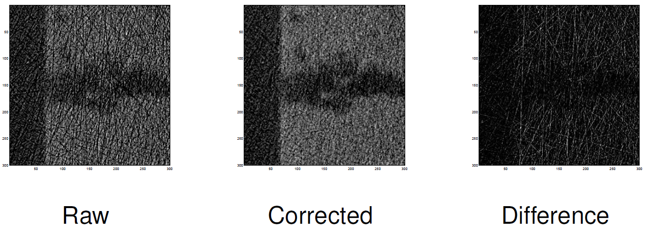
  • We should normalize the data
  • This was a raw projection, what happens if we use a flat field corrected image?
• Finds more spots than baseline
• Data is very unbalanced, try a selection of non-spot data for training.
  • Is it faster?
  • Is there a drop segmentation performance?

Note There are other spot detection methods that perform better than the baseline.

Clean up

del k_class

Convolutional neural networks for segmentation

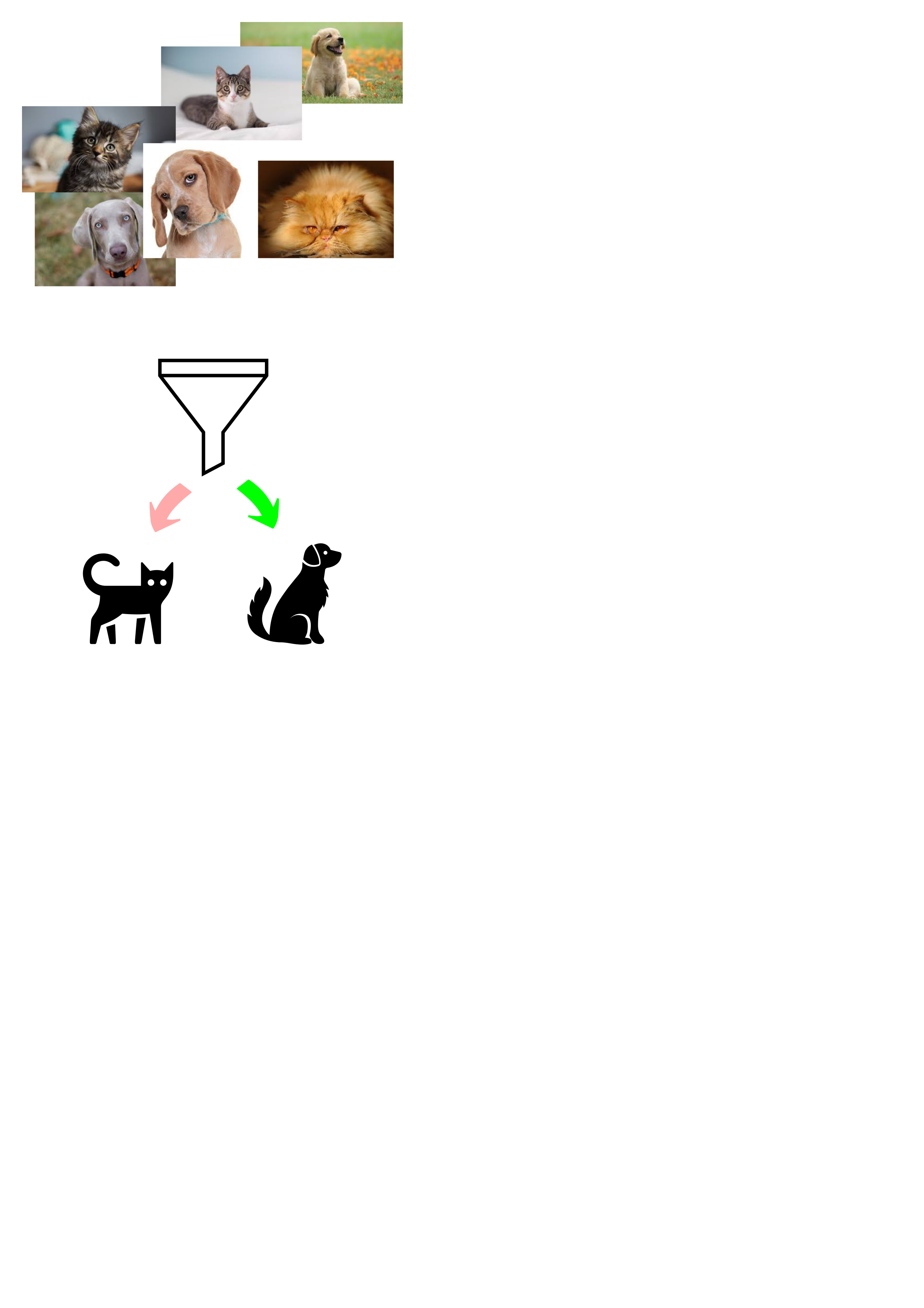
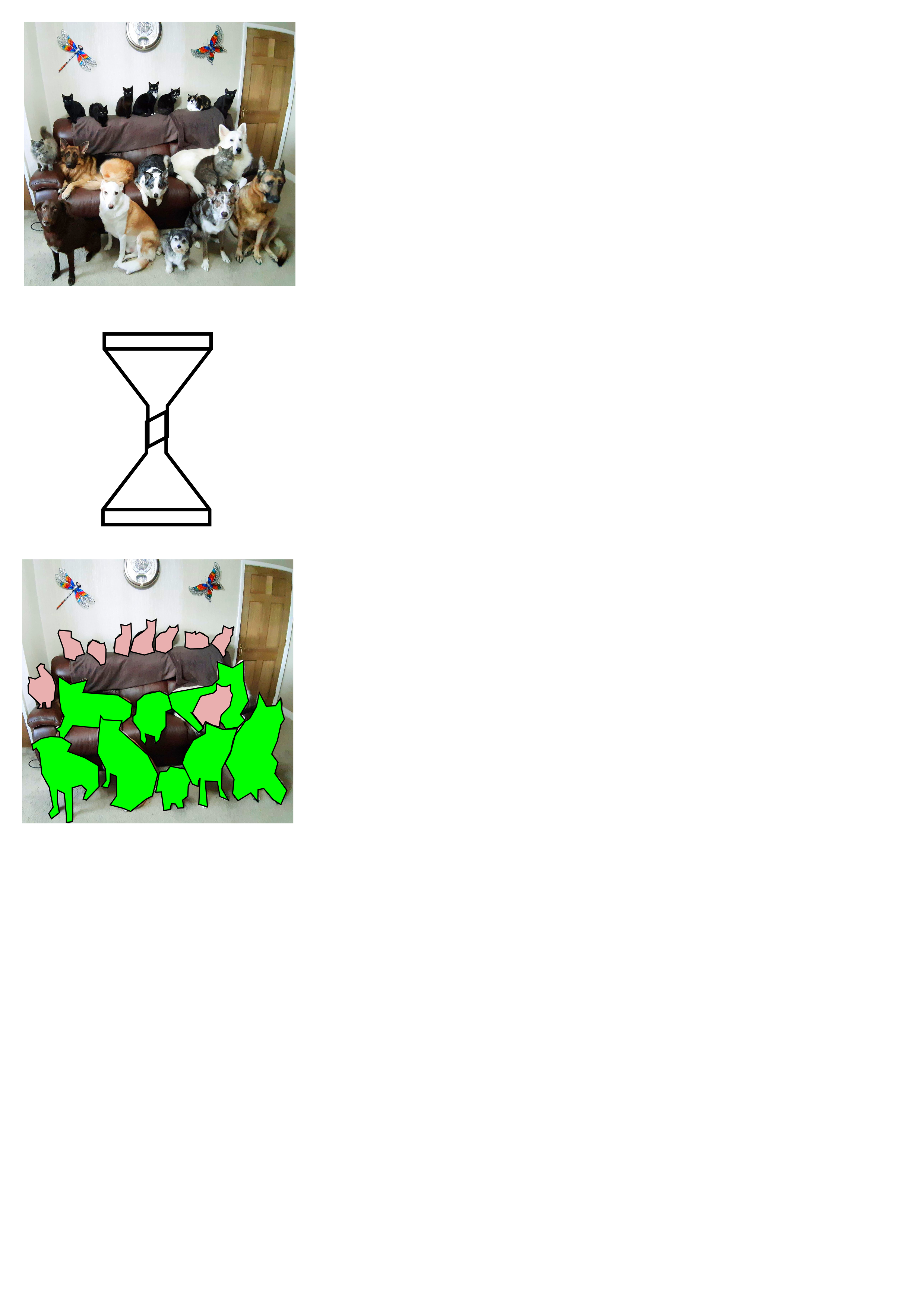
The difference between classification and segmentation I

Classification	Segmentation
pixels to classes	pixels to pixels

Network architecture Classification vs Segmentation

Classification	Segmentation

Different segmentation networks

Segmentation is mostly based on variations of the U-Net architechture

• AlexNET
• SegNET
• SegCaps

Scales in traditional image processing	U-Net architecture

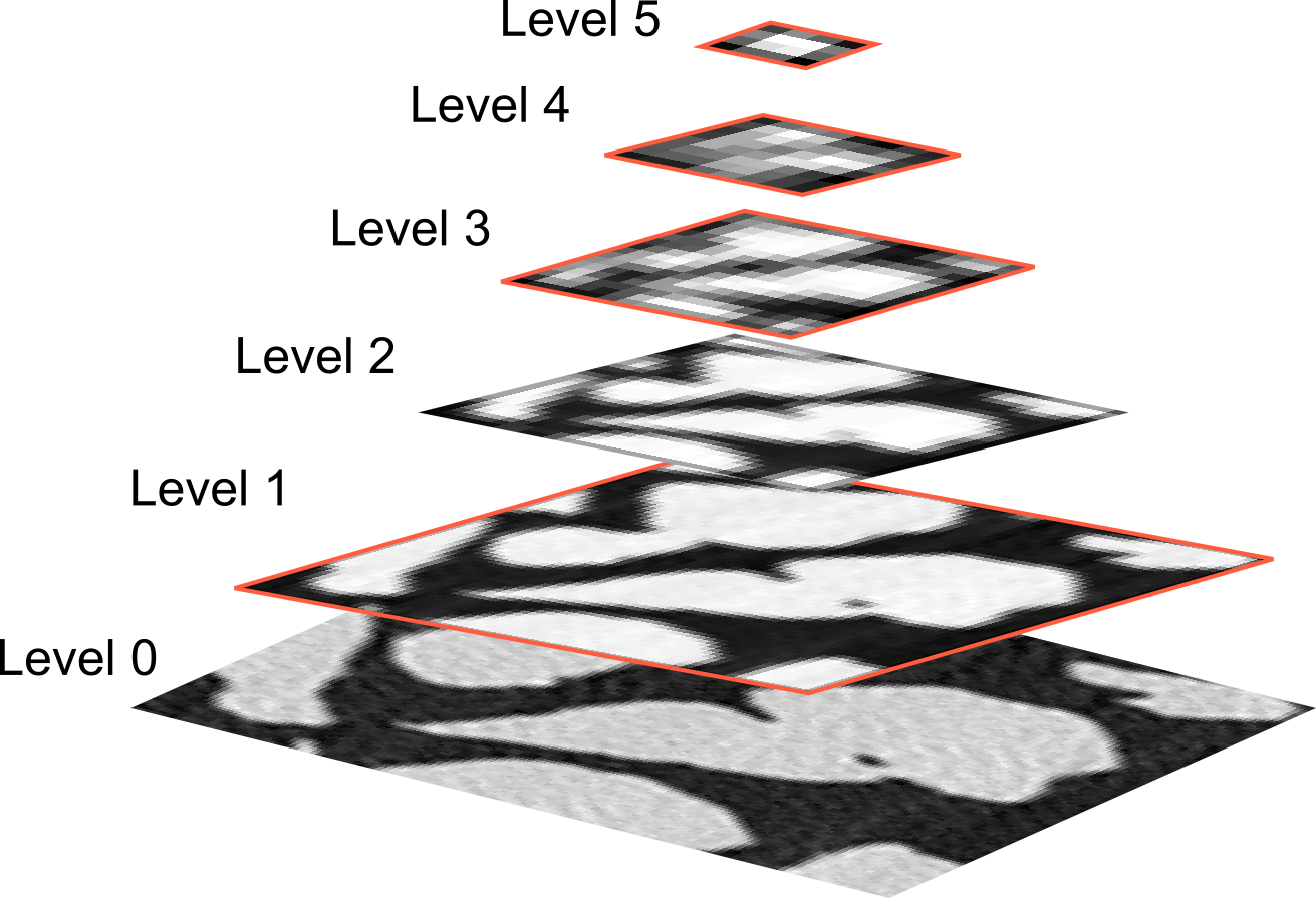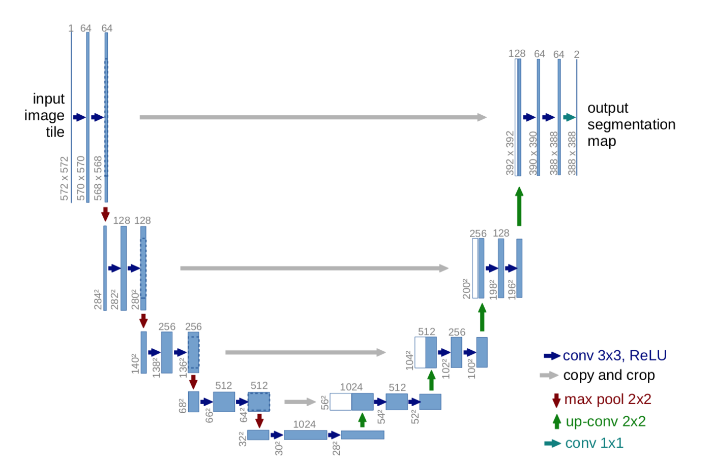Training data

We have two choices:

1. Use real data
   • requires time consuming markup to provide training data
   • corresponds to real life images
2. Synthesize data
   • flexible and provides both 'dirty' data and ground truth.
   • model may not behave as real data

Preparing real data

We will use the spotty image as training data for this example

There is only one image!

fig,ax=plt.subplots(1,2,figsize=(12,5))
ax[0].imshow(forig,vmin=0,vmax=4000,cmap='gray'); ax[0].set_title('Original');
ax[1].imshow(mask,cmap='gray'); ax[1].set_title('Mask');

Prepare training, validation, and test data

Any analysis system must be verified to be demonstrate its performance and to further optimize it.

For this we need to split our data into three categories:

1. Training data
2. Test data
3. Validation data

wpos = [1100,600]; ww   = 512
train_img,  valid_img, forigc = forig[128:256, 500:1300], forig[500:1000, 300:1500], forig[wpos[0]:(wpos[0]+ww),wpos[1]:(wpos[1]+ww)]
train_mask, valid_mask, maskc = mask[128:256, 500:1300],  mask[500:1000, 300:1500],  mask[wpos[0]:(wpos[0]+ww),wpos[1]:(wpos[1]+ww)]

fig, ax = plt.subplots(1, 4, figsize=(15, 6), dpi=300); ax=ax.ravel()

ax[0].imshow(train_img, cmap='bone',vmin=0,vmax=4000);ax[0].set_title('Train Image')
ax[1].imshow(train_mask, cmap='bone'); ax[1].set_title('Train Mask')
ax[2].imshow(valid_img, cmap='bone',vmin=0,vmax=4000); ax[2].set_title('Validation Image')
ax[3].imshow(valid_mask, cmap='bone');ax[3].set_title('Validation Mask');

The training image is as you probably already have noted very small. This is on purpose here to allow the training to run without introducing too long training times during the lecture. You will however see that the performance of the model is relatively good.

```{figure} figures/WorkflowWithValidationSet.pdf

scale: 100%

How the three data sets training, validation, and test are used when a network is trained and optimized. ```

Training	Validation	Test
70%	15%	15%

Build a CNN for spot detection and cleaning

We need:

• Data
  • Gray level image - our radiograph.
  • Annotated image where the spots are marked.
• A U-net model
  • Keras comes to our help

Build a U-Net model

def buildSpotUNet( base_depth = 48) :
    in_img = Input((None, None, 1), name='Image_Input')
    lay_1 = Conv2D(base_depth, kernel_size=(3, 3), padding='same',activation='relu')(in_img)
    lay_2 = Conv2D(base_depth, kernel_size=(3, 3), padding='same',activation='relu')(lay_1)
    lay_3 = MaxPooling2D(pool_size=(2, 2))(lay_2)
    lay_4 = Conv2D(base_depth*2, kernel_size=(3, 3), padding='same',activation='relu')(lay_3)
    lay_5 = Conv2D(base_depth*2, kernel_size=(3, 3), padding='same',activation='relu')(lay_4)
    lay_6 = MaxPooling2D(pool_size=(2, 2))(lay_5)
    lay_7 = Conv2D(base_depth*4, kernel_size=(3, 3), padding='same',activation='relu')(lay_6)
    lay_8 = Conv2D(base_depth*4, kernel_size=(3, 3), padding='same',activation='relu')(lay_7)
    lay_9 = UpSampling2D((2, 2))(lay_8)
    lay_10 = concatenate([lay_5, lay_9])
    lay_11 = Conv2D(base_depth*2, kernel_size=(3, 3), padding='same',activation='relu')(lay_10)
    lay_12 = Conv2D(base_depth*2, kernel_size=(3, 3), padding='same',activation='relu')(lay_11)
    lay_13 = UpSampling2D((2, 2))(lay_12)
    lay_14 = concatenate([lay_2, lay_13])
    lay_15 = Conv2D(base_depth, kernel_size=(3, 3), padding='same',activation='relu')(lay_14)
    lay_16 = Conv2D(base_depth, kernel_size=(3, 3), padding='same',activation='relu')(lay_15)
    lay_17 = Conv2D(1, kernel_size=(1, 1), padding='same',
                    activation='relu')(lay_16)
    t_unet = Model(inputs=[in_img], outputs=[lay_17], name='SpotUNET')
    return t_unet

Model summary

t_unet = buildSpotUNet(base_depth=24)
t_unet.summary()

WARNING:tensorflow:From /home/travis/miniconda/envs/book/lib/python3.7/site-packages/tensorflow_core/python/ops/resource_variable_ops.py:1630: calling BaseResourceVariable.__init__ (from tensorflow.python.ops.resource_variable_ops) with constraint is deprecated and will be removed in a future version.
Instructions for updating:
If using Keras pass *_constraint arguments to layers.
WARNING:tensorflow:From /home/travis/miniconda/envs/book/lib/python3.7/site-packages/keras/backend/tensorflow_backend.py:4070: The name tf.nn.max_pool is deprecated. Please use tf.nn.max_pool2d instead.

Model: "SpotUNET"
__________________________________________________________________________________________________
Layer (type)                    Output Shape         Param #     Connected to                     
==================================================================================================
Image_Input (InputLayer)        (None, None, None, 1 0                                            
__________________________________________________________________________________________________
conv2d_1 (Conv2D)               (None, None, None, 2 240         Image_Input[0][0]                
__________________________________________________________________________________________________
conv2d_2 (Conv2D)               (None, None, None, 2 5208        conv2d_1[0][0]                   
__________________________________________________________________________________________________
max_pooling2d_1 (MaxPooling2D)  (None, None, None, 2 0           conv2d_2[0][0]                   
__________________________________________________________________________________________________
conv2d_3 (Conv2D)               (None, None, None, 4 10416       max_pooling2d_1[0][0]            
__________________________________________________________________________________________________
conv2d_4 (Conv2D)               (None, None, None, 4 20784       conv2d_3[0][0]                   
__________________________________________________________________________________________________
max_pooling2d_2 (MaxPooling2D)  (None, None, None, 4 0           conv2d_4[0][0]                   
__________________________________________________________________________________________________
conv2d_5 (Conv2D)               (None, None, None, 9 41568       max_pooling2d_2[0][0]            
__________________________________________________________________________________________________
conv2d_6 (Conv2D)               (None, None, None, 9 83040       conv2d_5[0][0]                   
__________________________________________________________________________________________________
up_sampling2d_1 (UpSampling2D)  (None, None, None, 9 0           conv2d_6[0][0]                   
__________________________________________________________________________________________________
concatenate_1 (Concatenate)     (None, None, None, 1 0           conv2d_4[0][0]                   
                                                                 up_sampling2d_1[0][0]            
__________________________________________________________________________________________________
conv2d_7 (Conv2D)               (None, None, None, 4 62256       concatenate_1[0][0]              
__________________________________________________________________________________________________
conv2d_8 (Conv2D)               (None, None, None, 4 20784       conv2d_7[0][0]                   
__________________________________________________________________________________________________
up_sampling2d_2 (UpSampling2D)  (None, None, None, 4 0           conv2d_8[0][0]                   
__________________________________________________________________________________________________
concatenate_2 (Concatenate)     (None, None, None, 7 0           conv2d_2[0][0]                   
                                                                 up_sampling2d_2[0][0]            
__________________________________________________________________________________________________
conv2d_9 (Conv2D)               (None, None, None, 2 15576       concatenate_2[0][0]              
__________________________________________________________________________________________________
conv2d_10 (Conv2D)              (None, None, None, 2 5208        conv2d_9[0][0]                   
__________________________________________________________________________________________________
conv2d_11 (Conv2D)              (None, None, None, 1 25          conv2d_10[0][0]                  
==================================================================================================
Total params: 265,105
Trainable params: 265,105
Non-trainable params: 0
__________________________________________________________________________________________________

Functions to prepare data for training

def prep_img(x, n=1): 
    return (prep_mask(x, n=n)-train_img.mean())/train_img.std()


def prep_mask(x, n=1): 
    return np.stack([np.expand_dims(x, -1)]*n, 0)

Test the untrained model

Running the model without training is nothing you would normally do. Still, it may give you an indication if the model produces signal amplitudes that are relevant for the problem.

• We can make predictions with an untrained model (default parameters)
• but we clearly do not expect them to be very good

unet_pred = t_unet.predict(prep_img(forigc))[0, :, :, 0]

WARNING:tensorflow:From /home/travis/miniconda/envs/book/lib/python3.7/site-packages/keras/backend/tensorflow_backend.py:422: The name tf.global_variables is deprecated. Please use tf.compat.v1.global_variables instead.

fig, m_axs = plt.subplots(2, 3, figsize=(15, 6), dpi=150)
for c_ax in m_axs.ravel():
    c_ax.axis('off')
((ax1, _, ax2), (ax3, ax4, ax5)) = m_axs
ax1.imshow(train_img, cmap='bone',vmin=0,vmax=4000); ax1.set_title('Train Image')
ax2.imshow(train_mask, cmap='viridis'); ax2.set_title('Train Mask')

ax3.imshow(forigc, cmap='bone',vmin=0, vmax=4000); ax3.set_title('Test Image')
ax4.imshow(unet_pred, cmap='viridis', vmin=0, vmax=0.1); ax4.set_title('Predicted Segmentation')

ax5.imshow(maskc, cmap='viridis'); ax5.set_title('Ground Truth');

The untrained model doesn't perform very well. You clearly see that the image structures appear here. What is worth noting the spots already appear as amplified. This what we want to improve during the training.

Training conditions

The training is an iterative optmization process that tries to minimize a loss function. In this case we chose to use the ADAM optimizer to minimize the binary cross-correlation loss function. This loss function is often used for segmentation problems. The choice to the the training run for 20 epochs is rather a practical choice to allow the training to finish in reasonable time during the lecture. I leave it to you to try longer training sessions.

• Loss function - Binary cross-correlation
• Optimizer - ADAM
• 20 Epochs (training iterations)

During the training we will also record the history of different metrics to be able to observe the training behaviour.

• Metrics
  1. True positives
  2. False positives
  3. True negatives
  4. False negatives
  5. Binary accuracy (percentage of pixels correct classified) $$BA=\frac{1}{N}\sum_i(f_i==g_i)$$
  6. Precision $$Precision=\frac{TP}{TP+FP}$$
  7. Recall $$Recall=\frac{TP}{TP+FN}$$
  8. Area under reciever operating characteristics (ROC) curve $$AUC=\int ROC$$
  9. Mean absolute error $$MAE=\frac{1}{N}\sum_i|f_i-g_i|$$

Some of these metrics will turn out to be useless in this example. The reason is the class unbalanced in the data. The spots represent about 1% of the pixels in the image.

Compile the model

mlist = [
      metrics.TruePositives(name='tp'),        metrics.FalsePositives(name='fp'), 
      metrics.TrueNegatives(name='tn'),        metrics.FalseNegatives(name='fn'), 
      metrics.BinaryAccuracy(name='accuracy'), metrics.Precision(name='precision'),
      metrics.Recall(name='recall'),           metrics.AUC(name='auc'),
      metrics.MeanAbsoluteError(name='mae')]

t_unet.compile(
    loss=loss.BinaryCrossentropy(),  # we use the binary cross-entropy to optimize
    optimizer=opt.Adam(lr=1e-3),     # we use ADAM to optimize
    metrics=mlist                    # we keep track of the metrics in mlist
)

WARNING:tensorflow:From /home/travis/miniconda/envs/book/lib/python3.7/site-packages/keras/backend/tensorflow_backend.py:3172: where (from tensorflow.python.ops.array_ops) is deprecated and will be removed in a future version.
Instructions for updating:
Use tf.where in 2.0, which has the same broadcast rule as np.where

A general note on the following demo

This is a very bad way to train a model;

• the optimizer can be tweaked, e.g. the learning rate can be changed,
• the training and validation data should not come from the same sample (and definitely not the same measurement).
• a single image does not provide a good base for a general spot detection algorithm.

The goal is to be aware of these techniques and have a feeling for how they can work for complex problems.

Training the spot detection model

We train the model during 20 epochs using 3 samples per epoch. The optimizer uses the loss computed from a single validation image.

Nsamples = 3
Nepochs  = 20
loss_history = t_unet.fit(prep_img(train_img, n=Nsamples),
                          prep_mask(train_mask, n=Nsamples),
                          validation_data=(prep_img(valid_img),
                                           prep_mask(valid_mask)),
                          epochs=Nepochs,
                          verbose = 2)

Train on 3 samples, validate on 1 samples
Epoch 1/20
 - 10s - loss: 0.0885 - tp: 0.0000e+00 - fp: 0.0000e+00 - tn: 304656.0000 - fn: 2544.0000 - accuracy: 0.9917 - precision: 0.0000e+00 - recall: 0.0000e+00 - auc: 0.4037 - mae: 0.0407 - val_loss: 0.1122 - val_tp: 10.0000 - val_fp: 5.0000 - val_tn: 593511.0000 - val_fn: 6474.0000 - val_accuracy: 0.9892 - val_precision: 0.6667 - val_recall: 0.0015 - val_auc: 0.5409 - val_mae: 0.0206
Epoch 2/20
 - 7s - loss: 0.0929 - tp: 6.0000 - fp: 0.0000e+00 - tn: 304656.0000 - fn: 2538.0000 - accuracy: 0.9917 - precision: 1.0000 - recall: 0.0024 - auc: 0.5248 - mae: 0.0159 - val_loss: 0.1100 - val_tp: 23.0000 - val_fp: 13.0000 - val_tn: 593503.0000 - val_fn: 6461.0000 - val_accuracy: 0.9892 - val_precision: 0.6389 - val_recall: 0.0035 - val_auc: 0.5923 - val_mae: 0.0363
Epoch 3/20
 - 7s - loss: 0.0951 - tp: 12.0000 - fp: 0.0000e+00 - tn: 304656.0000 - fn: 2532.0000 - accuracy: 0.9918 - precision: 1.0000 - recall: 0.0047 - auc: 0.5822 - mae: 0.0280 - val_loss: 0.1010 - val_tp: 16.0000 - val_fp: 8.0000 - val_tn: 593508.0000 - val_fn: 6468.0000 - val_accuracy: 0.9892 - val_precision: 0.6667 - val_recall: 0.0025 - val_auc: 0.6288 - val_mae: 0.0215
Epoch 4/20
 - 7s - loss: 0.0853 - tp: 6.0000 - fp: 0.0000e+00 - tn: 304656.0000 - fn: 2538.0000 - accuracy: 0.9917 - precision: 1.0000 - recall: 0.0024 - auc: 0.6159 - mae: 0.0165 - val_loss: 0.1214 - val_tp: 10.0000 - val_fp: 2.0000 - val_tn: 593514.0000 - val_fn: 6474.0000 - val_accuracy: 0.9892 - val_precision: 0.8333 - val_recall: 0.0015 - val_auc: 0.6416 - val_mae: 0.0108
Epoch 5/20
 - 7s - loss: 0.0965 - tp: 3.0000 - fp: 0.0000e+00 - tn: 304656.0000 - fn: 2541.0000 - accuracy: 0.9917 - precision: 1.0000 - recall: 0.0012 - auc: 0.6263 - mae: 0.0083 - val_loss: 0.0993 - val_tp: 18.0000 - val_fp: 7.0000 - val_tn: 593509.0000 - val_fn: 6466.0000 - val_accuracy: 0.9892 - val_precision: 0.7200 - val_recall: 0.0028 - val_auc: 0.7299 - val_mae: 0.0112
Epoch 6/20
 - 7s - loss: 0.0812 - tp: 6.0000 - fp: 0.0000e+00 - tn: 304656.0000 - fn: 2538.0000 - accuracy: 0.9917 - precision: 1.0000 - recall: 0.0024 - auc: 0.7084 - mae: 0.0086 - val_loss: 0.0779 - val_tp: 76.0000 - val_fp: 36.0000 - val_tn: 593480.0000 - val_fn: 6408.0000 - val_accuracy: 0.9892 - val_precision: 0.6786 - val_recall: 0.0117 - val_auc: 0.7385 - val_mae: 0.0248
Epoch 7/20
 - 7s - loss: 0.0759 - tp: 36.0000 - fp: 6.0000 - tn: 304650.0000 - fn: 2508.0000 - accuracy: 0.9918 - precision: 0.8571 - recall: 0.0142 - auc: 0.6784 - mae: 0.0191 - val_loss: 0.0646 - val_tp: 162.0000 - val_fp: 123.0000 - val_tn: 593393.0000 - val_fn: 6322.0000 - val_accuracy: 0.9892 - val_precision: 0.5684 - val_recall: 0.0250 - val_auc: 0.8015 - val_mae: 0.0364
Epoch 8/20
 - 7s - loss: 0.0564 - tp: 93.0000 - fp: 48.0000 - tn: 304608.0000 - fn: 2451.0000 - accuracy: 0.9919 - precision: 0.6596 - recall: 0.0366 - auc: 0.7700 - mae: 0.0281 - val_loss: 0.0788 - val_tp: 218.0000 - val_fp: 219.0000 - val_tn: 593297.0000 - val_fn: 6266.0000 - val_accuracy: 0.9892 - val_precision: 0.4989 - val_recall: 0.0336 - val_auc: 0.8566 - val_mae: 0.0613
Epoch 9/20
 - 7s - loss: 0.0781 - tp: 147.0000 - fp: 93.0000 - tn: 304563.0000 - fn: 2397.0000 - accuracy: 0.9919 - precision: 0.6125 - recall: 0.0578 - auc: 0.8611 - mae: 0.0644 - val_loss: 0.0633 - val_tp: 191.0000 - val_fp: 127.0000 - val_tn: 593389.0000 - val_fn: 6293.0000 - val_accuracy: 0.9893 - val_precision: 0.6006 - val_recall: 0.0295 - val_auc: 0.8870 - val_mae: 0.0446
Epoch 10/20
 - 7s - loss: 0.0600 - tp: 123.0000 - fp: 54.0000 - tn: 304602.0000 - fn: 2421.0000 - accuracy: 0.9919 - precision: 0.6949 - recall: 0.0483 - auc: 0.8944 - mae: 0.0457 - val_loss: 0.0478 - val_tp: 148.0000 - val_fp: 67.0000 - val_tn: 593449.0000 - val_fn: 6336.0000 - val_accuracy: 0.9893 - val_precision: 0.6884 - val_recall: 0.0228 - val_auc: 0.8967 - val_mae: 0.0232
Epoch 11/20
 - 7s - loss: 0.0393 - tp: 90.0000 - fp: 33.0000 - tn: 304623.0000 - fn: 2454.0000 - accuracy: 0.9919 - precision: 0.7317 - recall: 0.0354 - auc: 0.8938 - mae: 0.0188 - val_loss: 0.0533 - val_tp: 108.0000 - val_fp: 32.0000 - val_tn: 593484.0000 - val_fn: 6376.0000 - val_accuracy: 0.9893 - val_precision: 0.7714 - val_recall: 0.0167 - val_auc: 0.8892 - val_mae: 0.0137
Epoch 12/20
 - 7s - loss: 0.0496 - tp: 66.0000 - fp: 18.0000 - tn: 304638.0000 - fn: 2478.0000 - accuracy: 0.9919 - precision: 0.7857 - recall: 0.0259 - auc: 0.8444 - mae: 0.0106 - val_loss: 0.0441 - val_tp: 127.0000 - val_fp: 42.0000 - val_tn: 593474.0000 - val_fn: 6357.0000 - val_accuracy: 0.9893 - val_precision: 0.7515 - val_recall: 0.0196 - val_auc: 0.9295 - val_mae: 0.0159
Epoch 13/20
 - 7s - loss: 0.0358 - tp: 84.0000 - fp: 27.0000 - tn: 304629.0000 - fn: 2460.0000 - accuracy: 0.9919 - precision: 0.7568 - recall: 0.0330 - auc: 0.9254 - mae: 0.0133 - val_loss: 0.0468 - val_tp: 136.0000 - val_fp: 47.0000 - val_tn: 593469.0000 - val_fn: 6348.0000 - val_accuracy: 0.9893 - val_precision: 0.7432 - val_recall: 0.0210 - val_auc: 0.8983 - val_mae: 0.0237
Epoch 14/20
 - 7s - loss: 0.0433 - tp: 90.0000 - fp: 27.0000 - tn: 304629.0000 - fn: 2454.0000 - accuracy: 0.9919 - precision: 0.7692 - recall: 0.0354 - auc: 0.8614 - mae: 0.0264 - val_loss: 0.0529 - val_tp: 145.0000 - val_fp: 54.0000 - val_tn: 593462.0000 - val_fn: 6339.0000 - val_accuracy: 0.9893 - val_precision: 0.7286 - val_recall: 0.0224 - val_auc: 0.8489 - val_mae: 0.0311
Epoch 15/20
 - 7s - loss: 0.0543 - tp: 93.0000 - fp: 33.0000 - tn: 304623.0000 - fn: 2451.0000 - accuracy: 0.9919 - precision: 0.7381 - recall: 0.0366 - auc: 0.7918 - mae: 0.0382 - val_loss: 0.0532 - val_tp: 142.0000 - val_fp: 50.0000 - val_tn: 593466.0000 - val_fn: 6342.0000 - val_accuracy: 0.9893 - val_precision: 0.7396 - val_recall: 0.0219 - val_auc: 0.8291 - val_mae: 0.0302
Epoch 16/20
 - 7s - loss: 0.0549 - tp: 93.0000 - fp: 33.0000 - tn: 304623.0000 - fn: 2451.0000 - accuracy: 0.9919 - precision: 0.7381 - recall: 0.0366 - auc: 0.7748 - mae: 0.0383 - val_loss: 0.0525 - val_tp: 129.0000 - val_fp: 41.0000 - val_tn: 593475.0000 - val_fn: 6355.0000 - val_accuracy: 0.9893 - val_precision: 0.7588 - val_recall: 0.0199 - val_auc: 0.8227 - val_mae: 0.0259
Epoch 17/20
 - 7s - loss: 0.0509 - tp: 78.0000 - fp: 27.0000 - tn: 304629.0000 - fn: 2466.0000 - accuracy: 0.9919 - precision: 0.7429 - recall: 0.0307 - auc: 0.7772 - mae: 0.0324 - val_loss: 0.0515 - val_tp: 121.0000 - val_fp: 34.0000 - val_tn: 593482.0000 - val_fn: 6363.0000 - val_accuracy: 0.9893 - val_precision: 0.7806 - val_recall: 0.0187 - val_auc: 0.8337 - val_mae: 0.0205
Epoch 18/20
 - 7s - loss: 0.0453 - tp: 75.0000 - fp: 21.0000 - tn: 304635.0000 - fn: 2469.0000 - accuracy: 0.9919 - precision: 0.7812 - recall: 0.0295 - auc: 0.8012 - mae: 0.0242 - val_loss: 0.0528 - val_tp: 112.0000 - val_fp: 28.0000 - val_tn: 593488.0000 - val_fn: 6372.0000 - val_accuracy: 0.9893 - val_precision: 0.8000 - val_recall: 0.0173 - val_auc: 0.8621 - val_mae: 0.0147
Epoch 19/20
 - 7s - loss: 0.0414 - tp: 66.0000 - fp: 15.0000 - tn: 304641.0000 - fn: 2478.0000 - accuracy: 0.9919 - precision: 0.8148 - recall: 0.0259 - auc: 0.8439 - mae: 0.0150 - val_loss: 0.0555 - val_tp: 107.0000 - val_fp: 26.0000 - val_tn: 593490.0000 - val_fn: 6377.0000 - val_accuracy: 0.9893 - val_precision: 0.8045 - val_recall: 0.0165 - val_auc: 0.8866 - val_mae: 0.0114
Epoch 20/20
 - 7s - loss: 0.0403 - tp: 66.0000 - fp: 15.0000 - tn: 304641.0000 - fn: 2478.0000 - accuracy: 0.9919 - precision: 0.8148 - recall: 0.0259 - auc: 0.8855 - mae: 0.0091 - val_loss: 0.0545 - val_tp: 118.0000 - val_fp: 27.0000 - val_tn: 593489.0000 - val_fn: 6366.0000 - val_accuracy: 0.9893 - val_precision: 0.8138 - val_recall: 0.0182 - val_auc: 0.8903 - val_mae: 0.0117

Training history plots

During the training you could see that the metrics we asked for change values. The values can be reviewed after training to evaluate if the model performs well.

titleDict = {'tp': "True Positives",'fp': "False Positives",'tn': "True Negatives",'fn': "False Negatives", 'accuracy':"BinaryAccuracy",'precision': "Precision",'recall':"Recall",'auc': "Area under Curve", 'mae': "Mean absolute error"}

fig,ax = plt.subplots(2,5, figsize=(20,8), dpi=300)
ax =ax.ravel()
for idx,key in enumerate(titleDict.keys()): 
    ax[idx].plot(loss_history.epoch, loss_history.history[key], color='coral', label='Training')
    ax[idx].plot(loss_history.epoch, loss_history.history['val_'+key], color='cornflowerblue', label='Validation')
    ax[idx].set_title(titleDict[key]); 

ax[9].axis('off');
axLine, axLabel = ax[0].get_legend_handles_labels() # Take the lables and plot line information from the first panel
lines =[]; labels = []; lines.extend(axLine); labels.extend(axLabel);fig.legend(lines, labels, bbox_to_anchor=(0.7, 0.3), loc='upper left');

Prediction on the training data

unet_train_pred = t_unet.predict(prep_img(train_img[:,wpos[1]:(wpos[1]+ww)]))[0, :, :, 0]

fig, m_axs = plt.subplots(1, 3, figsize=(18, 4), dpi=150); m_axs= m_axs.ravel(); 
for c_ax in m_axs: c_ax.axis('off')

m_axs[0].imshow(train_img[:,wpos[1]:(wpos[1]+ww)], cmap='bone', vmin=0, vmax=4000), m_axs[0].set_title('Train Image')
m_axs[1].imshow(unet_train_pred, cmap='viridis', vmin=0, vmax=0.2), m_axs[1].set_title('Predicted Training')
m_axs[2].imshow(train_mask[:,wpos[1]:(wpos[1]+ww)], cmap='viridis'), m_axs[2].set_title('Train Mask');

Prediction using unseen data

unet_pred = t_unet.predict(prep_img(forigc))[0, :, :, 0]

fig, m_axs = plt.subplots(1, 3, figsize=(18, 4), dpi=150); m_axs = m_axs.ravel() ; 
for c_ax in m_axs: c_ax.axis('off')
m_axs[0].imshow(forigc, cmap='bone', vmin=0, vmax=4000); m_axs[0].set_title('Full Image')
f1=m_axs[1].imshow(unet_pred, cmap='viridis', vmin=0, vmax=0.1); m_axs[1].set_title('Predicted Segmentation'); fig.colorbar(f1,ax=m_axs[1]);
m_axs[2].imshow(maskc,cmap='viridis'); m_axs[2].set_title('Ground Truth');

Converting predictions to segments

fig, ax = plt.subplots(1,2, figsize=(12,4))
ax0=ax[0].imshow(unet_pred, vmin=0, vmax=0.1); ax[0].set_title('Predicted segmentation'); fig.colorbar(ax0,ax=ax[0])
ax[1].imshow(0.05<unet_pred), ax[1].set_title('Final segmenation');

Hit cases

gt = maskc
pr = 0.05<unet_pred
ps.showHitCases(gt,pr,cmap='gray')

Hit map

ps.showHitMap(gt,pr)
plt.savefig('spotunet.png')

Comparing the performance of the spot detection methods

Baseline

k-NN

U-Net

Concluding remarks about the spot detection

• Spot detection seems to be working well using the U-Net.
• A great amount of the spots are found.
• There are many false positive pixels - usually in the neighborhood of a spot.
• Some misclasifications are probably related to the annotation of the training image.
• Wide spot items may be related to the network depth.
• The demo sample is smooth, we didn't test the performance near edges

Improvements

• Increase the number of epochs in the training
• Increase the training data
  • Add images with different SNR (real and simulated)
  • Add images with different characteristics

Segmenting root networks in the rhizosphere

Background

• Soil and in particular the rhizosphere are of central interest for neutron imaging users.
• The experiments aim to follow the water distribution near the roots.
• The roots must be identified in 2D and 3D data

Today: much of this mark-up is done manually!

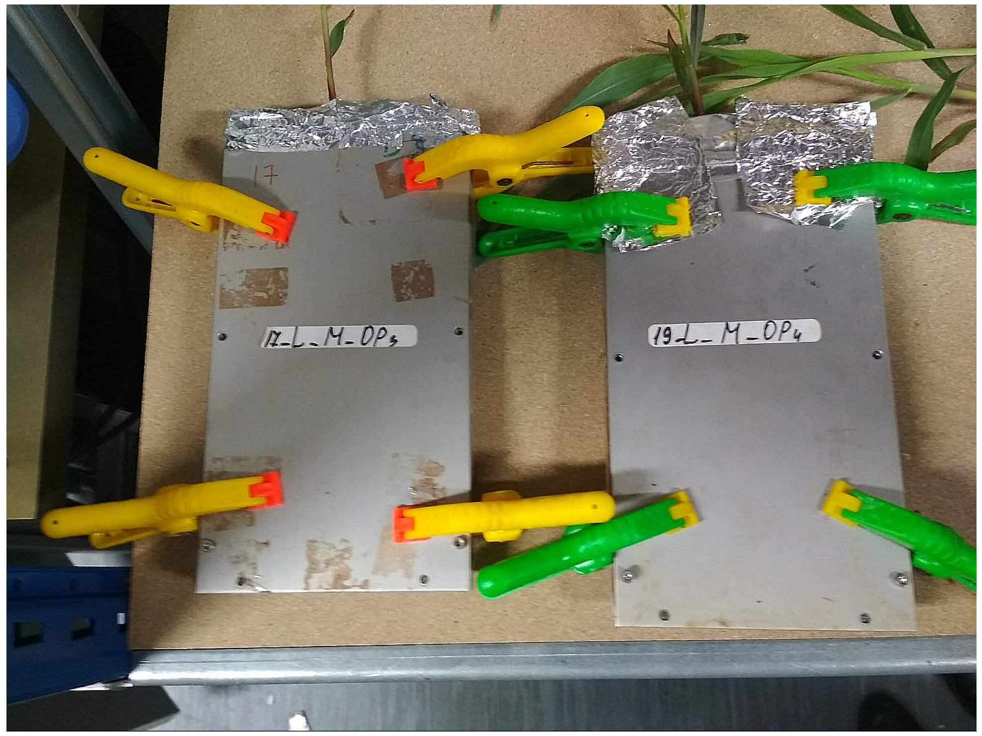
Acknowledgement: This work was done by Gian Guido Parenza as a master project.

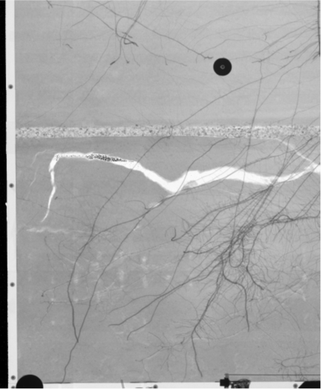
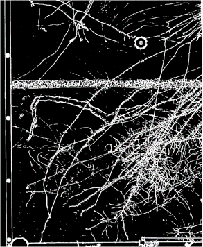
Available data

Radiography	Tomography
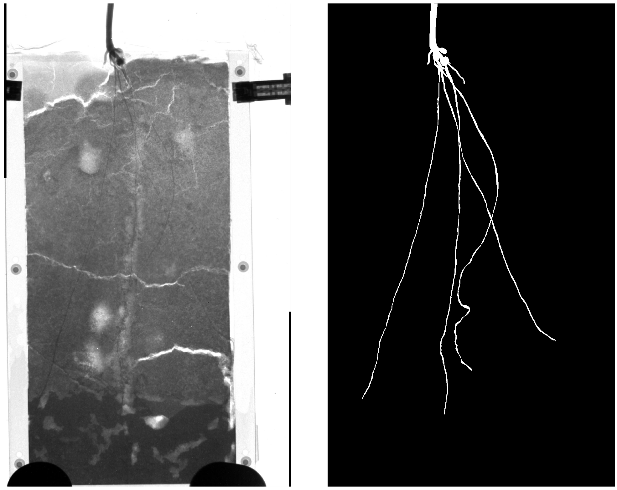Provided by A. Carminati et al.	Provided by M. Menon et al.

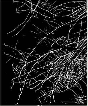
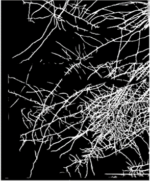
Results using current method

Radiograph of a rhizobox	Current segmentation

Problems: Unwanted elements are marked as roots

1. Elements of the container
2. Soil cracks
3. The porous barrier

Workflow

```{figure} figures/roots/GraphicalAbstract_03.pdf

scale: 100%

The rhizospere experiment and analysis workflow. ```

Considered NN model

This task is again a good case for the U-Net model

Training

	Radiography	Tomography
Data size	256x256	64x64x64
Training times	2-3 min/epoch	30-40 min/epoch

Loss functions

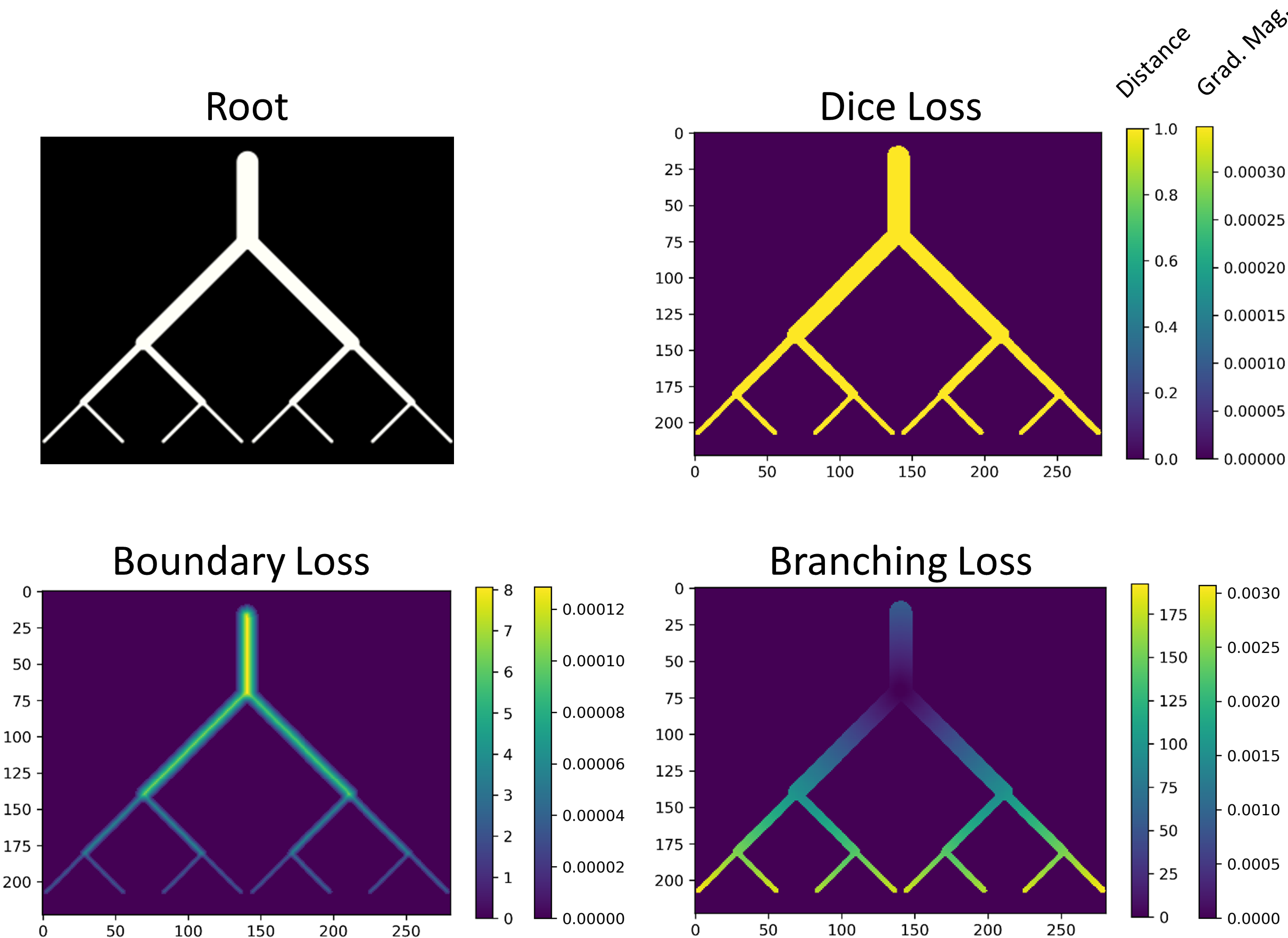
The impact of different loss functions

Compare different loss functions	Details of branching loss

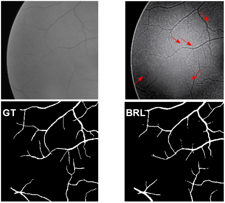Transfer learning

• We have little available annotated neutron data
  • There is more radiographs than tomograms

Our options

• Simulations using root network simulators and Monte Carlo neutron simulation
• Use data with similar features.

Medical image processing is the saviour!

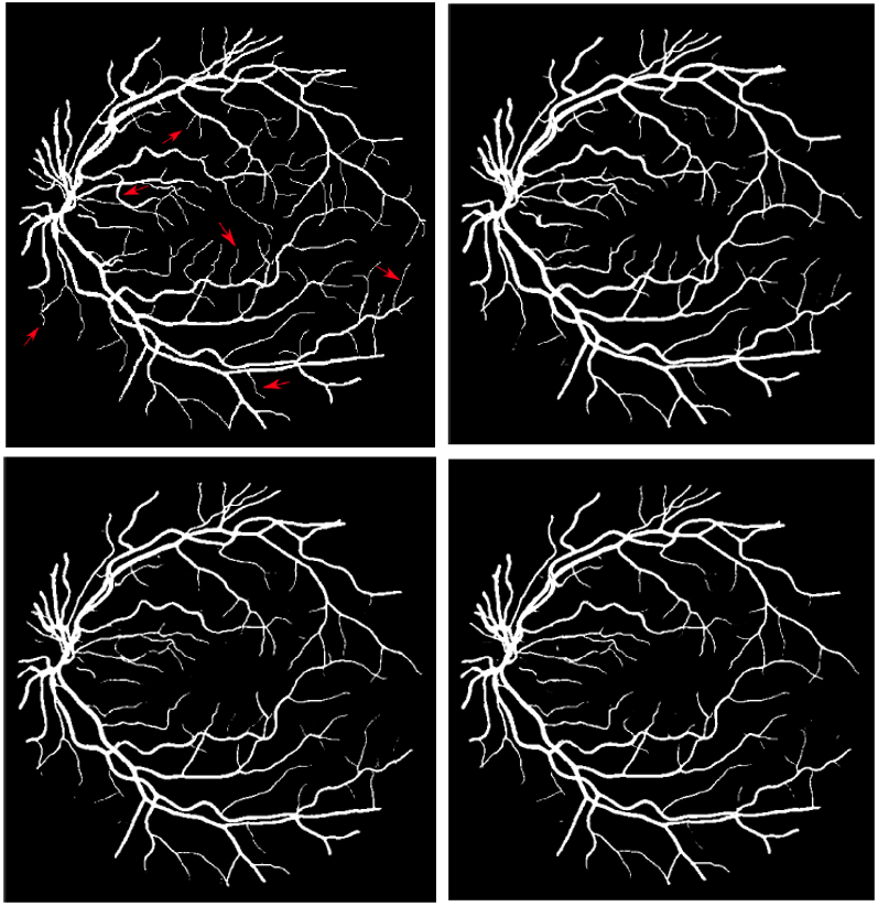
Trying transfer learning on the roots

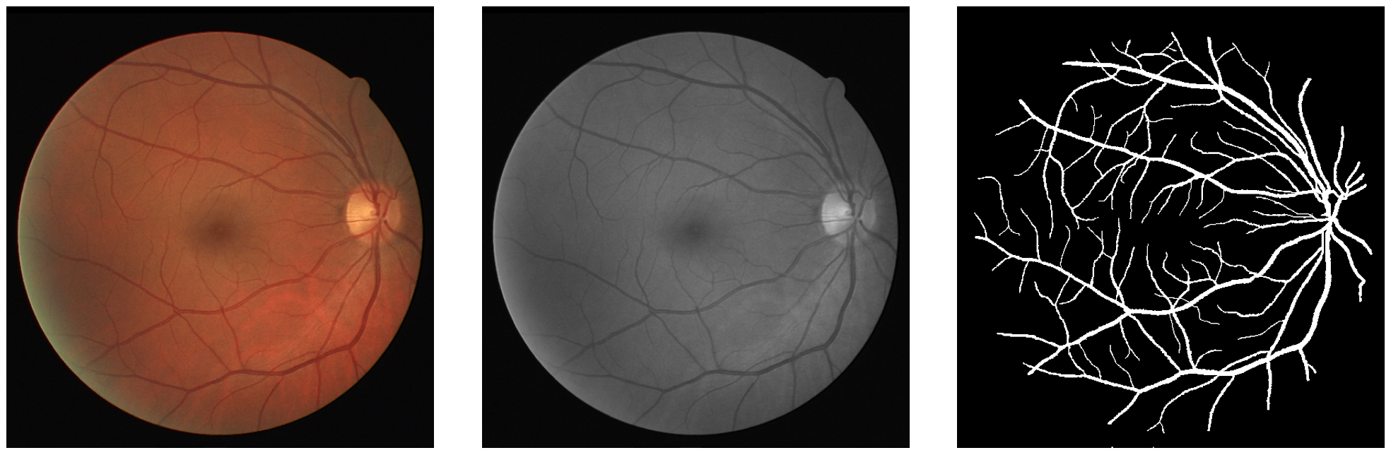
U-Net trained with roots only	U-Net trained with transfer learning

Transfer learning

• Speeds up the training with root data
• Improves the segmented results
• Can even be used for 3D data

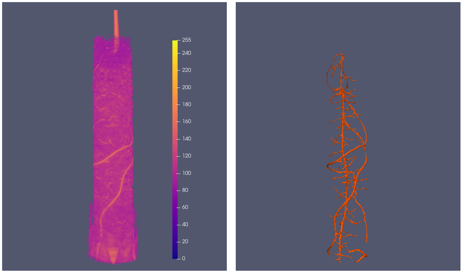
The model can also be used for volume data

after some modification

Original tomography data and ground truth	Segmentations

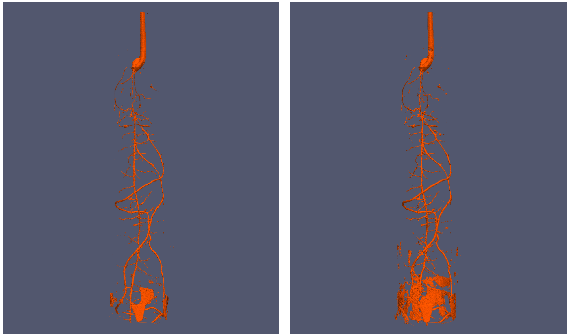Summary

This project has shown that

• Convolutional NNs can segment roots in soil
• Will save a lot of work in future rhizospere experiment

The models still need more training to cover wider variations in the data.

Concluding remarks

We have demonstrated how some machine learning techniques can be used on neutron images:

• Some background to the segmentation problem and neutron imaging
• k-means - to segment ToF spectra
• Spot detection
  • Baseline algorithm
  • k-Nearest neighbors
  • U-Net
• Root segmentation
  • U-Net
  • Different loss metrics
  • Training performance